Help MawisGeoportal

MawisGeoportal is used to visualize, manage and analyze geodata in one place. It is a convenient tool for creating new documentation and managing existing geodata and documents.
The geoportal functionality is divided into modules. Only those modules that have been made available to you by the administrator (have been purchased) are available in your Geoportal. You do not need to have all modules available.
The following modules/tools are possible in the application:
- Map Layer Organizer - Tool for enabling/disabling layers in project and map
- Export map - Allows to export the map to selected formats
- Search - This is a general data search. You can search in address point data, cadastre data or data layers
- Measurements - Tool for map measurements and saving them
- Katastr- It is used to search for parcels as polygons and offers a wider range of possibilities to work with results in table form and also to whisper existing cadastres.
- Tabular data - Used to work with spatial data attributes
- Taskmanager - Task list with the possibility of assigning tasks to a user and notifications of status changes
- 3D Models - Tool for displaying and registering all 3D models in the project
- Expression Support - Module used to support expressions about the existence of networks
The application is divided into 2D and 3D data display. When switching to 3D, the Map Layer Organizer and Map Export modules are available
There are video tutorials for the application:
- Videos - Videos about Mawis Geoportal applications, modules and their usage
Mawis Services Team
Copyright © 2024-2026 HRDLIČKA spol. s r.o. - All rights reserved
+420 251 618 458 (Mon-Fri 8:00-16:00) | info@mawis.eu
 If the application does not behave as described in the Help, we recommend that you first clear the cache of your web browser. MGM is developed and tested on current versions of Google Chrome, Microsoft Egde and Mozilla Firefox
Google Chrome: https://support.google.com/accounts/answer/32050?co=GENIE.Platform%3DDesktop&hl=cs
Microsoft Edge: https://support.microsoft.com/cs-cz/help/10607/microsoft-edge-view-delete-browser-history
Mozilla Firefox:https://support.mozilla.org/cs/kb/jak-vymazat-mezipamet
General application controls
1. GENERAL APPLICATION CONTROL
The Geoportal is divided into three basic parts/panels:
- Work panel - contains basic controls
- Display panel - displays data (e.g. attribute data or 3D)
- Map Window - displays spatial data
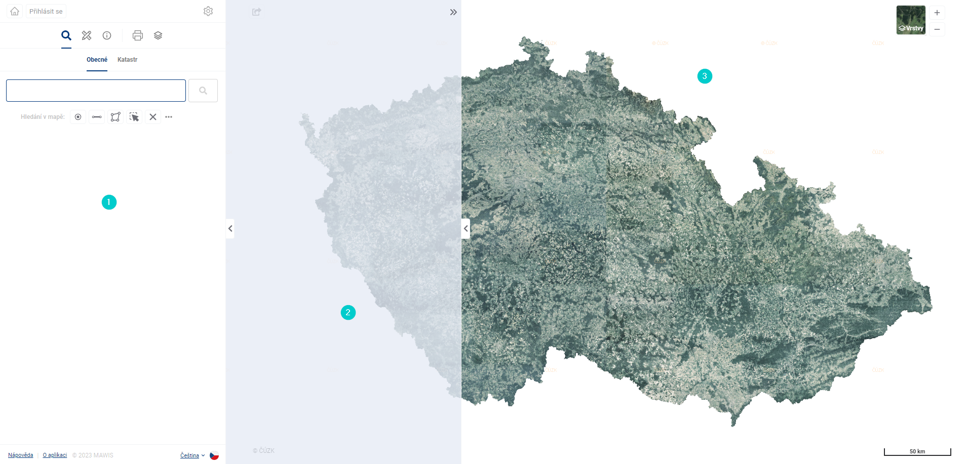
The panels can be customised to suit your needs. By dragging the edge of the panel you can expand, minimize and maximize the working and display panel. The display panel is activated only when the data display tools are activated (For example, after displaying the search result detail or clicking on the 3D Model).
Login and projects
1.1. APPLICATIONS AND PROJECTS
When the Geoportal is first loaded, the user is presented with a public project with the basic functions of the application. To use MGM fully, you must first purchase the product and then log in. To purchase the product, please feel free to contact us.
You can log in to the geoportal in the top bar of the work panel using the “Log in” button. 
To successfully log in, you must have purchased the product and be registered here. After pressing the “Login” button, you must fill in the user’s email and password.
If you forget your password, you can reset it directly in the login window. A temporary password will be sent by email and the next time you log in, you will be prompted to set a new password.

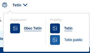
After a successful login, the user icon, the organization icon, and the user’s default project are displayed in the upper left corner of the application. To switch between projects, you need to go to the project name bar.
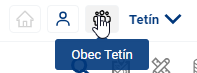
The user will see all his available configured projects. To configure a new project, please contact us.
Work panel
1.2. WORKING PANEL
The work panel allows basic control of the geoportal and work with data. The user can search the data, work with cadastral data, perform measurements and especially view and edit attribute data.
The work panel is divided into four sections:
- UPPER FOX

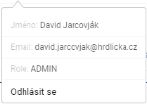
In this part of the work panel, the user can log in and view basic information about the logged-in user (name, email and role). Alternatively, it is possible to log out of the application.
After logging in, the user is shown the available geoportal projects and can switch between them. (See chapter 1.2 Login and projects)
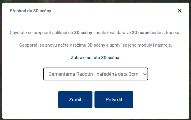
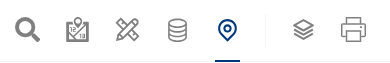
In the right part of the bar there is a switch  between 2D and 3D state of the project, you can switch to 3D only when the project includes a 3D scene. When clicked, a dialog box will appear with a selection of the scene you want to switch to.
- TOOLBAR

The toolbar displays the available tools for the project. The tools vary depending on the project the user is logged in to and the license/module purchased. For example, in a public project without login, the following tools are available:
- General search
- Measurements
- Layer organiser
- Map export.
The individual geoportal tools and their options are described in detail in the following chapters.
Other available toolbar functionalities vary according to the selected tool that the user has active. The active tool is underlined in the toolbar. In this section, the actual work with data, search, measurement and more takes place.
- WORK PANEL FOOT

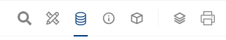
In the footer of the working panel, you can find the application help, contact to the customer centre, information about the application and its current version and the possibility to switch between the available MGM languages.
Display panel
1.3. DISPLAY PANEL
This panel is mainly used for data display. The display panel is always activated after the data display action has been initiated. For example, a request to open a parcel detail in a general search.
The display panel can show detailed information about the registered objects, or possibly also 3D models (Module “3D Models”).
In the display panel it is also possible to upload, remove and view previews of files attached to registered objects using the Gallery.
Map window
1.4. MAP WINDOW
The map window can be intuitively navigated using the mouse and zoomed using the mouse wheel or the + and - buttons. The button in between returns the map window to its default position, i.e. to the zoom and centering level when the project is opened.
The mouse wheel can also be used to move the map (by clicking and dragging) in case the drawing is currently started and the left mouse button would draw and not move.

Spatial data and underlying or user layers are displayed in the map window. The contents of the map window can be easily changed in the “Layer Organizer” (See chapter 2. Map Layer Organizer).
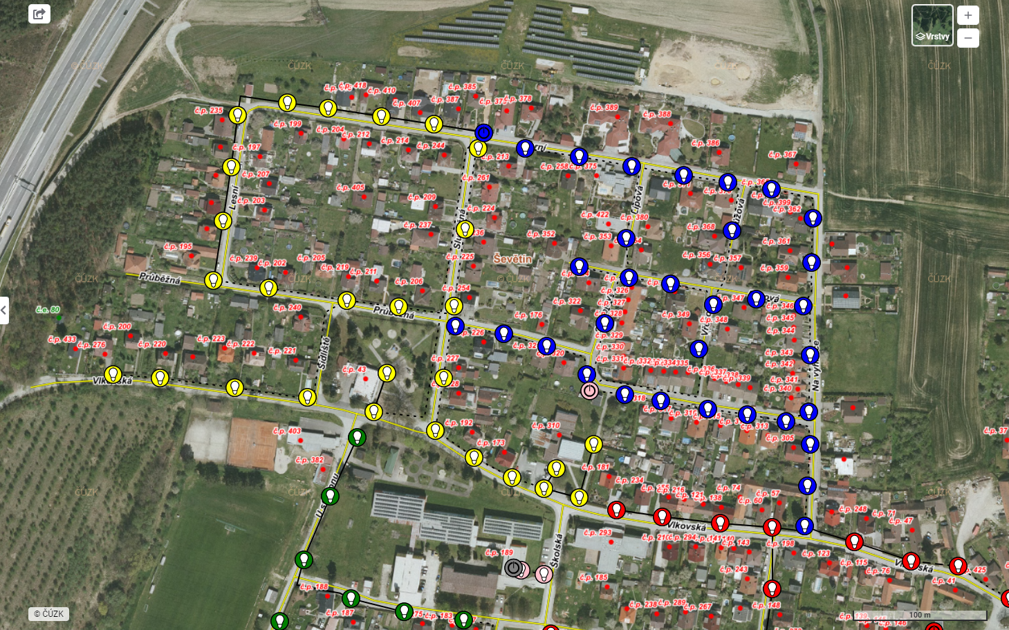
- the Project data layers are displayed according to the logged-in user and the selected project. This can display technical administrator maps, DTMs, passports and others that are stored in the geoportal database or connected via WMS. The image below shows the lighting passport.
-
User layers = layers of search, drawings and temporary user imports.
-
Basemap is set according to customer requirements. By default, the project is accompanied by an orthophotomap and a base map from ČÚZK.
To change the active base map, you can simply change the active base map directly in the top right corner of the map window.
There is also a button to turn on/off the positioning of the device on which the application is running. 
The contents of the map window can also be easily exported using the tool in the upper right corner. You can directly save the map window as a .PNG image, create a link to share the created image or quickly download it. Such an image or link can be sent by the application user to colleagues or saved for future use.

Another map window tool is Go to Panorama mapy.com/Google maps. After activating it, it is possible to click into the map and this will open a new tab in the browser with a panoramic view/map in mapy.com in the selected location or a view into Gogle Streetview/map, depending on the specific settings of the project.
The map window also displays the graphical scale (in the lower right corner) and the copyright of the external services used (in the lower left corner).
By pressing SHIFT and dragging the mouse at the same time, you can quickly zoom to the selected area. 
3D Map Window
1.5. MAP WINDOW 3D
Movement and rotation in the scene is done by using all mouse buttons (clicking and dragging) or by combination with the SHIFT key
Posun
- while holding the left mouse button, move the mouse left/right → move along the X-axis and towards/ away from you → move forward/backwards along the Y-axis
- while holding the right mouse button, the mouse can be moved left/right again → scroll on the X-axis and up/down → scroll on the Z-axis
Rotation The camera can be dynamic (rotating around the subject) or static (rotating the view in place).
- while holding the mouse wheel, the view rotates around the object at a distance determined by the mouse cursor position
- holding the left mouse button together with the SHIFT key can rotate the camera in place - the equivalent of looking around in reality
Proximity/distance
- when moving the mouse wheel, you can zoom in and out in the model
- the camera zooms in/out to a point below the cursor, not to the centre of the screen
- zoom allows passage through the model
Map Layer Organizer
2nd ORGANIZER OF MAP LINKS
In the Layer Organizer, you can activate and deactivate the layers displayed in the map field and display their legend.
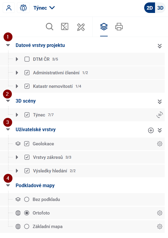
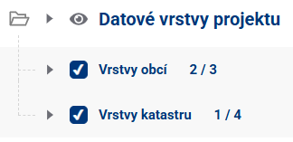
CATEGORIZATION OF MAP LAYERS
Map layers are divided into four basic groups in the application, and these can be further divided into thematic groups (for example, into passport layers).
ACTIVATE/DEACTIVATE LAYERS
- click on the check mark next to the layer name to activate/deactivate the selected layer in the map
- when activated, the parent groups are activated at the same time
- deactivation has no effect on the parent groups
- clicking on the checkmark next to the layer group name activates/deactivates the selected group in the map, which affects the visibility of subordinate layers
- by clicking on the check mark together with the CTRL key next to the layer group name, the subordinate elements in the lower levels are activated/deactivated in the map at the same time
- click on the checkbox next to the text Project data layers to activate/deactivate all connected data layers
- if the group is collapsed, an indicator appears showing how many child elements are active and how many are deactivated
QUESTIONING IN THE MAP
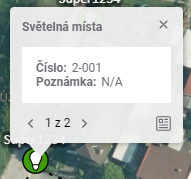
Some Data and User Layers can be queried by clicking into the map, which loads the attributes of the data layers into the Popup. This allows the user to easily find out all the details of the queryable layers at the point where they click. If there are multiple elements at a location, it is possible to scroll between them in the popup window.
the Popup window offers, besides the attributes of the item in question, also a button to go to the form and the possibility to copy the coordinates of the click point to the clipboard.
Layer pollability depends, among other things, on the visibility of the layer. It is not possible to click into the map to query elements of a layer that is disabled or invisible at the current zoom level.
LEGEND AND SETTINGS
Most layers have a legend with the symbols used and additional tools for zooming, navigating to the table and setting transparency. The legend makes it easier to identify elements in the map field. The user displays it by using the  button next to the layer.
A single layer can have multiple symbologies and categories within the symbology that can be independently turned on and off, similar to layers and layer groups.
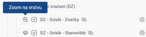
The “Zoom to Layer” tool zooms the map window so that all elements of the layer are visible. At the same time, the other layers will be temporarily muted to make the zoomed layer stand out better
You can quickly zoom into the layer range without opening the settings by hovering over the map base symbol next to the layer name
The “Go to table” tool redirects the user to the table of elements in the “Table data” module.
The “Transparency Settings” tool changes the transparency of the layer using a slider.
Data layers
2.1. DATA LAYERS
Data layers are the first of three categories in the Map Layer Organizer.
Common characteristics of Data layers:
- Elements can contain attributes that can be interacted with in the Table Data module;
- Specific to the project;
- They are hierarchically grouped;
- They have an available legend symbol ;
- They are inserted into the project by the administrator;
- Data layers can have their visibility set to scale. The gray colored layers in the workbench are not visible for a given scale level and will be displayed when the scale level is changed to a visible level.
User layers
2.2. USER-LAYERS
User layers are the second of three categories in the Map Layer Organizer
Common characteristics of User Layers:
- Their content is created by the user in the modules Search, Measurement and Taskmanager, or by temporary import of own data;
- Available for every project;
- They are hierarchically grouped.
Categorization:
- Layers of drawings - measurement and search drawings are written into them
- Search Results - contains the results of Search
- Taskmanager layer - a layer showing the task layouts from the taskmanager module in the map
- Custom Layers - temporary user import from file, layer disappears after leaving the project
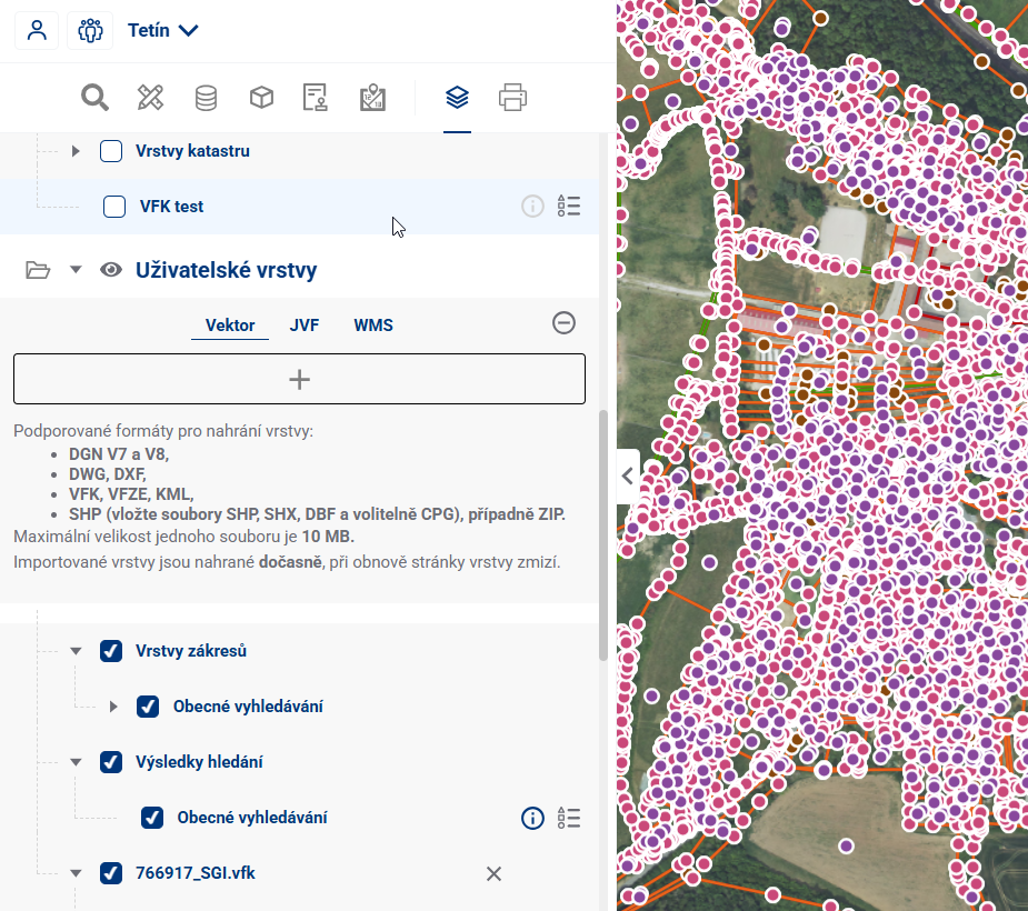
- If enabled by the project administrator, the user can use the
 button to add custom temporary layers
 - It is possible to upload Vector layers (DGN V7 and V8, DWG, DXF, VFK, VFZE, KML and SHP (insert three files SHP, SHX, DBF and optionally CPG), or ZIP), a JVF file, a georeferenced PDF with vector data and a URL to connect to the WMS layer
- There are size limits for uploaded files (10 Mb for vector and 30 Mb for JVF)
- After successful upload, the layer is displayed in the layer tree and can be worked with similarly to Data layers
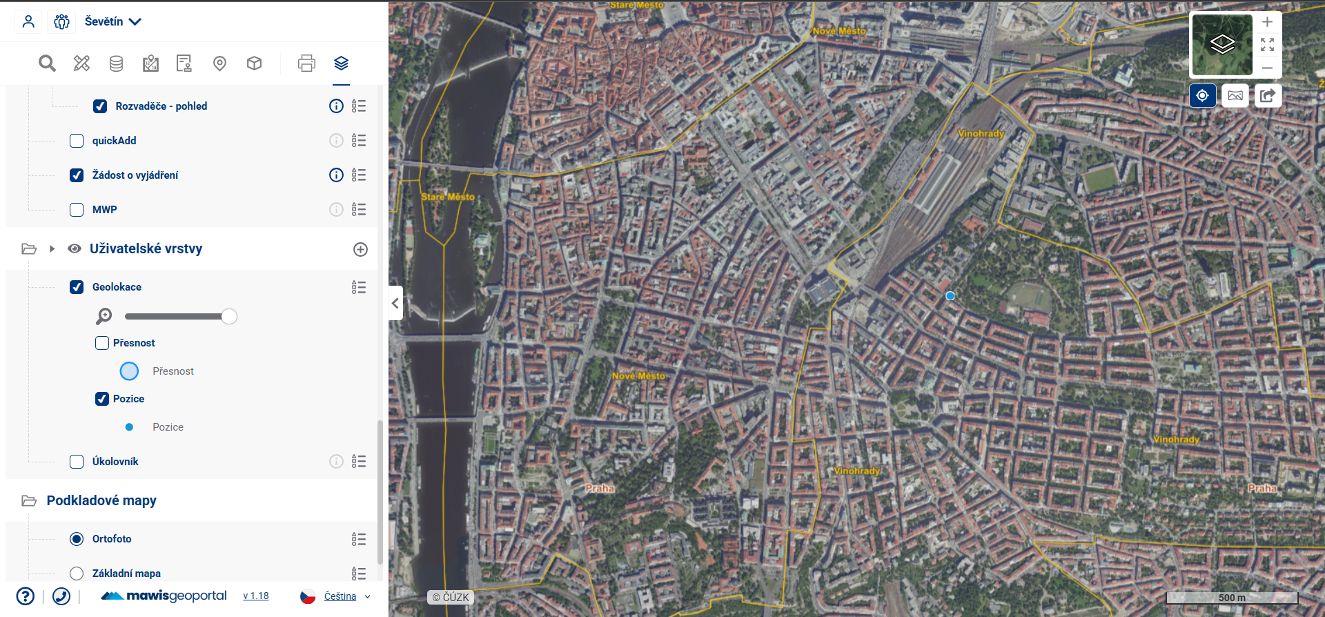
- If enabled by the project administrator, the user can use the
- Geolocation - layers displaying the targeting accuracy, the current position of the user (his device) and his orientation, enabled on the top right by
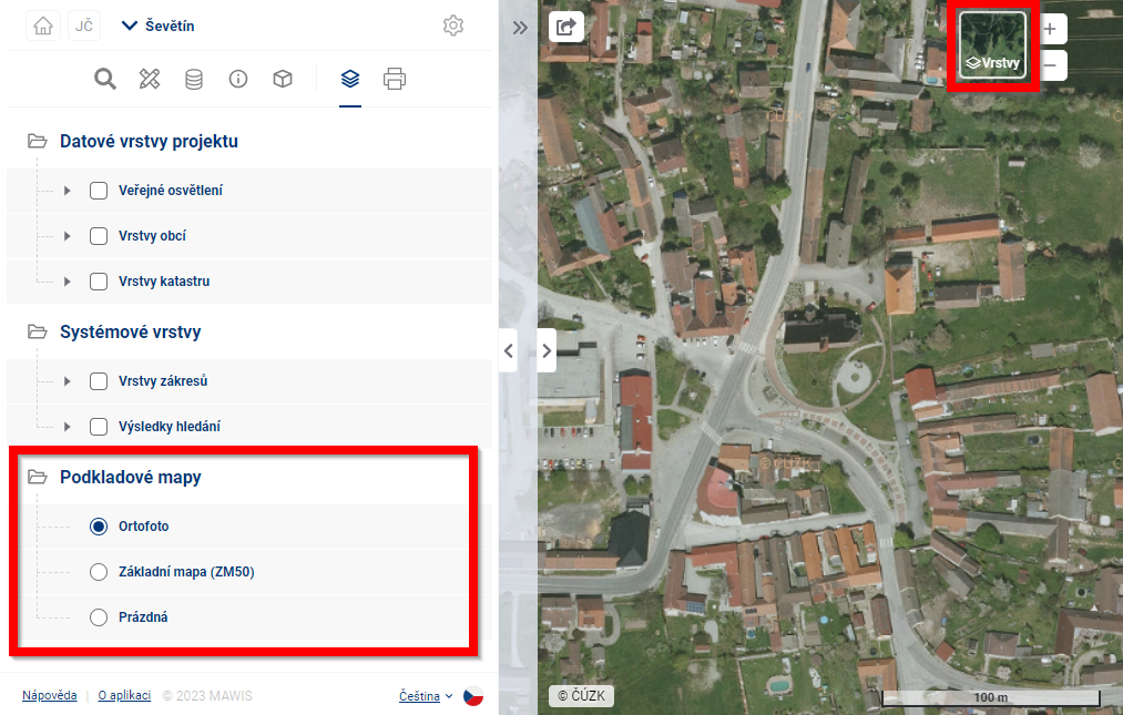
Background maps
2.3. BASE MAPS
Base maps are the last category in the Map Layer Organizer.
Common characteristics of the Background maps:
- They add a general positional map to the map field;
- They facilitate geographical orientation;
- You cannot interact with their symbols;
- Primarily it is a mapping service ČÚZK, any underlying maps can be added according to the customer’s requirements;
- The underlying maps can also be accessed via the menu at the top right of the map box.
Default base maps:
- Orthophoto - a real landscape image composed of aerial imagery in an orthophoto display;
- Base map of the Czech Republic 1:50 000 - topographic map of medium scale containing a position, elevation and description;
- Empty base map/No base map - turns off the display of base maps.
3D scenes
2.4. 3D Scenes
- 3D scenes contain data viewable after switching to 3D
- each scene can contain several layers, which together form the whole 3D model
- in 2D, each layer is represented by a purple polygon that shows the 2D footprint of the 3D model
- next to the scene title there is a button to go to the scene in 3D
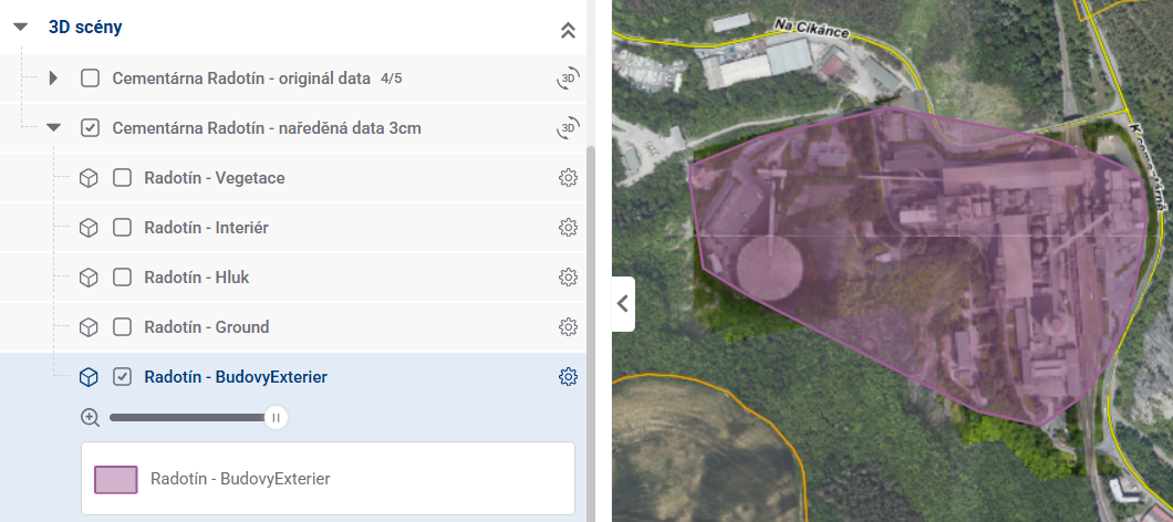
- individual layers can also be switched on and off in 3D
Map export
3. EXPORT MAPS
The Export Maps module is used to easily and quickly print maps from the Mawis Geoportal. The user can save or share the printed map.
In the module’s work panel, you can set map field parameters, out-of-frame data, and file options.
Instead of a traditional map field, a live preview of the printed map is displayed on a standardized A-size paper surface. The map content is generated according to the previously set map layers in the Map Layer Organizer. The user can switch between the modules without losing any adjustments in the map settings. By grabbing the map field and dragging with the left mouse button, or zooming using the mouse wheel, the displayed area can be fine-tuned.
SETTING MAP OUTPUT
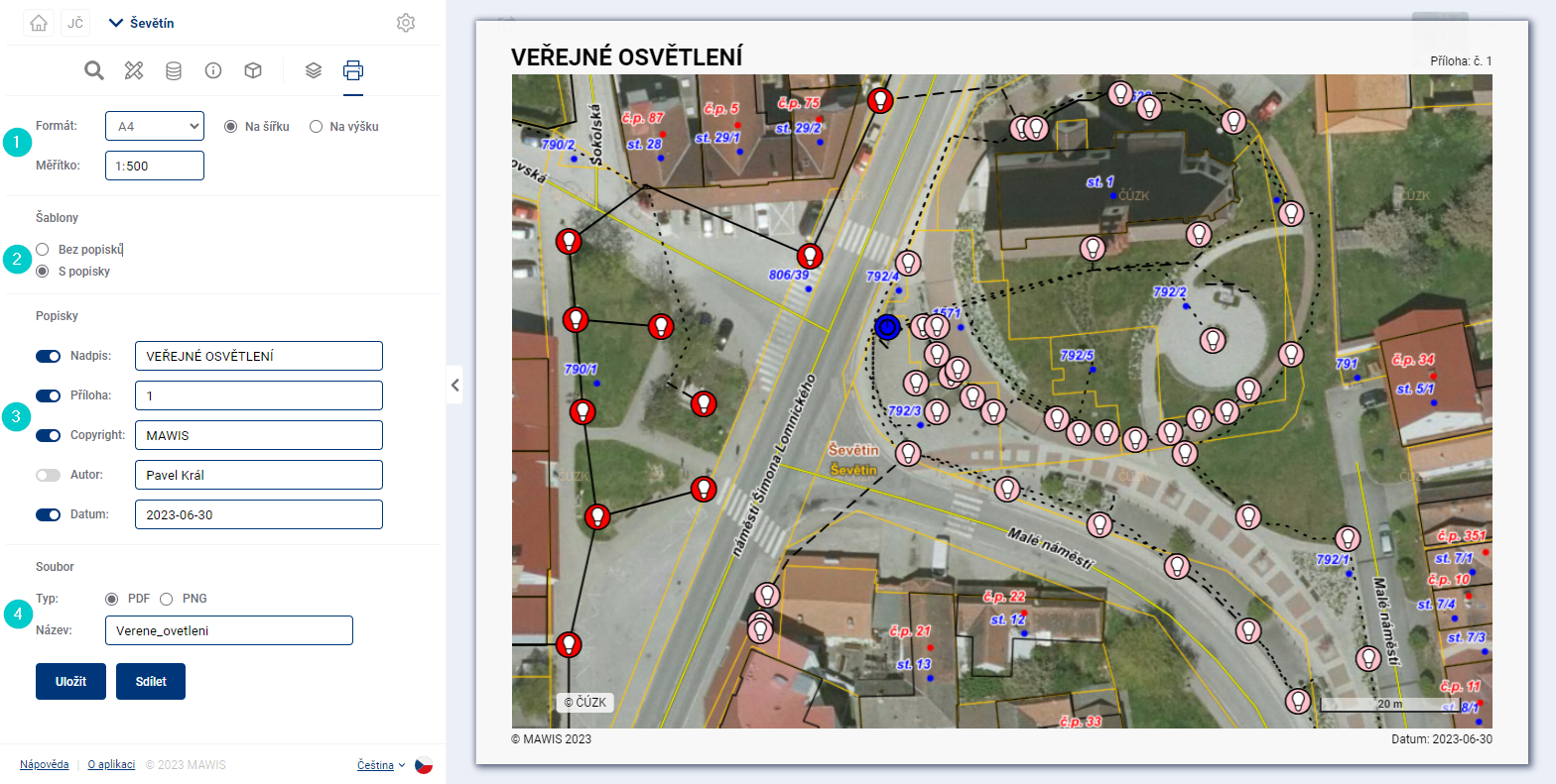
1. Format and scale
The user has a choice of standardised A3, A4 or A5 paper sizes with portrait or landscape orientation. The scale can be set virtually anywhere.
It is recommended to choose the format and scale according to the size, shape of the area and the desired level of detail or your own priorities. To maintain clarity, map markers should not overlap too much. The map can always be divided into several sheets. The scale is by convention a round number with a zero at the end.
2. Templates
You can set whether the map field will cover the entire sheet or whether any out-of-frame data will be added in the output frame.
The map frame is recommended e.g. if the map is intended for printing. A map without a frame may be suitable if the aim is only to record the current map field display in an image.
3. Out-of-frame data
In the left part you can set the out-of-frame data to be displayed on the map. The text field in the left part is used to write your own title, attachment number, author’s name, etc. In case of a copyright, the application will automatically add the current year.
The map title is normally written in capital letters.
4. Pictures
Whether it is possible to turn on and off the images to be included in the map. This can be for example a legend or a company logo. The menu of images and their size and position in the print window is determined by the configuration, so you need to contact the project administrator.
5. File
In the last section of the settings, you can choose whether to save a PDF or PNG file and specify a file name. Finally, you just need to use the button to save the map to a file or share it. In the case of sharing, a link can be copied to allow anyone with an internet connection to download the exported map.
Search
4. SEARCH
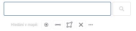
The general search displays address locations, parcel definition points and features from Data Layers in the map window based on a simple text or spatial search. When it is opened, a text search box is available and a spatial search toolbar below it.
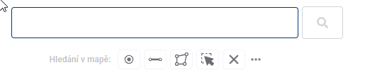
- Text search
For a simple text search, just type the desired text or part of the text into the specified field and press Enter or click the Magnifying glass icon. By clicking on the cross in the right part of the field, you can easily delete the field contents and search results.
Search results are sorted from the closest result according to the current location on the map.
Spatial search
The spatial search toolbar consists of the following tools:
- Point selection - allows you to plot one or more points on the map
- Line selection - used to draw lines
- Polygon selection - used to draw polygons
- Selection of drawn elements - by clicking on the previously drawn element you can select the element
- Delete drawn shape - deletes the selected shape or all drawn shapes at once
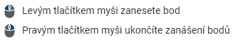
Drawing of shapes is done by clicking into the map, where for line and polygon each click adds a new break point of the element, clicking left and right mouse button on the same place will end the drawing, in case of polygon it will close it at the same time. Shapes can be edited by moving the breakpoints and by adding a new breakpoint to the line. A breakpoint can also be removed by pressing and holding the “CTRL” key and clicking on the selected point.
While it is possible to have different shapes drawn in the map window at the same time, the selection is only possible with one geometry type per search. Which geometry type will be used can be seen in the text box. The search is performed again by clicking on the magnifying glass icon.
Spatial search can be combined with text search. For example, you can search for all address locations containing a certain text in a plotted area.
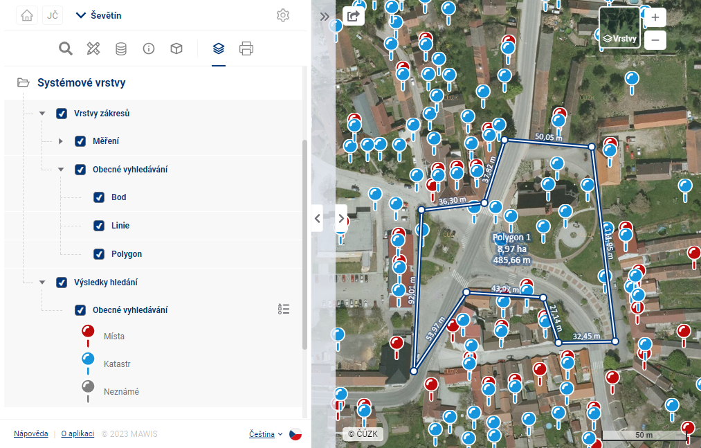
Working with results
The records retrieved by the search are then displayed in the workbench under the search tools. These results can then be filtered according to whether it is an address location (red), a parcel from the cadastre (blue) or an element from the data layers (green), zoom the map to the selected points using the magnifying glass icon and highlight the element in the map by hovering the mouse over the record in the work panel.
Clicking on an item in the Workbench will highlight the point in the map window and open a pop-up menu with details. The Cadastre data can also be displayed in the Display Panel using the “i” icon included in the record in the Work Panel or the icon in the bottom right corner of the popup, while the data for the search results in the data layers (Evidence) will open in the Work Panel when the icon is clicked.
Click on a search result in the map to see the basic details in a pop-up window. Double-clicking on a search point in the map also displays the point details in the viewport.
Measurements
5th MEASUREMENT
Home
The Measurement module is a standard part of all projects in the Mawis Geoportal. It is used to obtain coordinates and measure distances and areas on the map. It is a space where the user can easily add their own drawing to the map composition and then export it with tabular data with coordinates, distances and annotations.
Access to the module
- The module is accessible via the pencil icon crossed with the ruler in the project main bar
- The module designation is “Measurement”
There is a menu for drawing points, lines, areas and notes, which will be described in more detail below. The expansion menu below the three dots on the right allows you to decide whether to display text descriptions and measured values for the drawn features in the map window.
Module functions
The module includes the possibility to draw and manage 4 basic types of geometric elements:
Each geomteria type is also managed by a separate measurement results table
- Ability to create and manage all types of geometric elements
- Elements are displayed on the map and in the spreadsheet
- Option to Export marked data into a table or SHP file (shapefile)
- Ability to share data with other users
Manage layer visibility
- Access via Layer Organiser
- In the “User Layers” section you will find:
- Layers of drawings
- Measurement point
- Line measurement
- Measuring polygon
- Measurement note
- Layers of drawings
- Possibility of switching on/off individual layers
Working with data
Types of data storage
-
Temporary elements
- Marked with a clock icon
- Disappears after closing the application
-
Saved for users
- Only available for logged in user
- It will appear the next time you log in
-
Saved for everyone
- Visible to all project users
- Suitable for sharing and collaboration
Tabular display
- Search in records
- Filtering by columns
- Tagging of records
- Zooming in on selected features on the map (magnifying glass with plus sign)
- Delete records (trash icon) see Measurement results table
Data export
- Export to spreadsheet
- Export to SHP file (shapefile)
- It is used, for example, to send to the data manager for adding to the map in the project’s persistent layers.
Permanent data storage
- Temporary layers can only be converted to permanent layers via the administrator
- Elements saved “for me” and “for all” are available in user layers
- Access via the “Drawing layers” section by geometry type
Use for collaboration
- Suitable for information exchange between processors and users
- Possibility of commenting and commenting on the records
- Sharing via link with other project users
Point
5.1. POINT
Custom waypoints are added to the map by simply clicking anywhere in the map window after going to the measurement module. This creates an entry in the measurement results table. For each point, the table displays its S-JTSK coordinates as well as a name that the user can edit as desired. The position of the points can also be adjusted by simply dragging the point to another location in the map window.

Lines
5.2. LINES
After switching to line drawing mode, you can add broken lines to the map. Drawing is done by each click adding a new refraction point to the element, then double-clicking to finish drawing the element along with creating the point. A right click will also end the drawing, but at the previous point. A new click at a different point will start drawing the next line. Shapes can be edited by moving breakpoints and by adding a new breakpoint to the line. A breakpoint can also be removed by pressing and holding the “CTRL” key and clicking on the selected point.
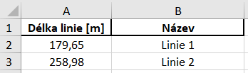
The results table contains a name that can be customized by the user and an indication of the measured line length. The partial lengths of the line segments between the breakpoints are shown on the map directly next to the line.
Polygon
5.3. POLYGONEM
After switching to polygon drawing mode, closed broken lines can be added to the map. Drawing is done by each click adding a new refraction point to the feature, double-clicking then closes the polygon by connecting the click point to the start point and finishing the feature drawing. A right click also ends the drawing, but without creating a new point at the click point. A new click at a different point will start drawing the next line. Shapes can be edited by moving breakpoints and by adding a new breakpoint to the line. A breakpoint can also be removed by pressing and holding the “CTRL” key and clicking on the selected point.
The results table contains a name, which the user can customize, and the measured perimeter and area of the shape. The partial lengths of the line segments between the breakpoints are shown on the map directly next to the line.
Note
5.4. POZNÁMKA
Adding point annotations works identically to adding points by simply clicking anywhere in the map window. The difference is in the appearance of the symbol and the attributes listed in the table. Again, it contains a name, which the user can customize, and which is displayed on the map, but in addition, it is possible to fill in an additional text column Note, for example with some additional comment, but which will no longer be visible on the map. Again, the position of points can be adjusted by simply dragging the point to another location in the map window.
Table of measurement results
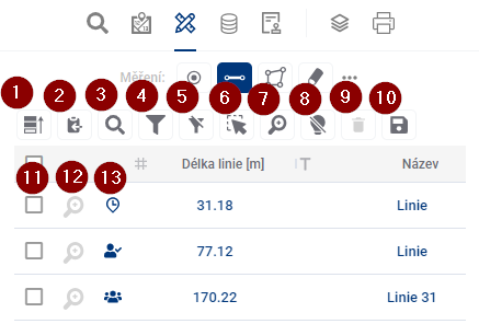
5.5 MEASUREMENT RESULTS TABLE
Each of the drawing variants - points, lines, polygons and annotations have their own results table, although they are displayed simultaneously in the map window and switching between them is the same as switching between drawing tools in the work panel under the module switcher. There is a group of tools above the table for controlling the results table and another directly in the table.
- Prioritize Selected - moves selected elements in the table before others
- Save selected to clipboard - and then you can paste the records into a text editor
- Search in data - a quick way to filter records using the text you enter
- Show/hide filter - show/hide text boxes to filter results for all columns
- Show only filtered in map - limits the visibility of features in the map to only those that are filtered
- Select map elements - allows you to select and highlight artwork by interacting with the map
- Browse to selected features - zooms to the selected features in the map window
- Disable highlighting of selected items
- Delete row - removes selected records from the results table. If none is selected, removes all of them.
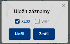
- Export selected data - allows you to export the results table to a selected format, for example .xlsx
- Select item in table - click in the check box to select and highlight the record
- Browse to feature - zooms to the selected feature drawing in the map window
- Save item - allows you to save measurements for yourself or for all users of the project
Select and highlight elements
When you hover over a row in the table, the row is highlighted and the drawing is highlighted in light blue in the map window.
The selected elements are highlighted in dark blue in the table and in the map and can be selected either by checking the checkbox on the left side of the table or by clicking on the shape in the map window, but only with the Select elements in map function enabled (Button 6). It is possible to use the polygon drawing to select multiple elements. Clicking and dragging draws a rectangle, single clicks allow you to create a polygon of any shape. Drawing is terminated by double-clicking or right-clicking. Prioritize Selected (Button 1) places the selected elements at the top of the table.
Approaching the elements
Zooming the map to the elements can be achieved in two ways. Browse to selected elements (Button 7) zooms the map to the elements that are selected and therefore highlighted in the table, Browse to element (Button 12), located next to each record, zooms the map to that particular element.
Filtering elements
Element filtering allows you to display only those records in the results table whose attribute meets a certain condition. The easiest and fastest way to do this is to use the Search in Data tool (Button 3), which displays a text box to enter the desired constraint. Filters for all columns separately can be accessed using Show/Hide Filter (Button 4), and for each column you can still open a popup with a more detailed filter specification and change the operator from “equals” to “is greater than”, for example.
Save data to file
Selected rows from the table can be saved to a file outside MGM in two different ways. A quicker solution can be achieved by using Save Selected to Clipboard (Button 2) and then pasting into, for example, an .xlsx file. The result then looks as follows:
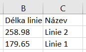
An alternative is Save Rows (Button 7), which allows saving records to a selected format - for example .xlsx or to a Shapefile file with geometry.

Save data for other users
The recorded measurement and annotation elements can be saved for future use using Save element (Button 13), which offers either saving only for the logged-in user or also for other project users. Of course, it is possible to leave an element unsaved, in which case it will disappear when the project is closed.
Cadastre
6th KATASTR
The cadastre search is used to search for parcels as polygons and offers a wider range of options for working with the results in table form and also whispering. It is an extension of the basic module Search;. The results of both search methods are independent of each other and can be switched between them seamlessly without fear of losing search results.
There are 2 ways to search. Either by typing the searched names or cadastre or parcel numbers into the search engine, or again by spatial search. You can combine these options and display the results together in one table.
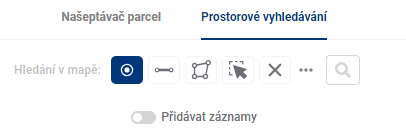
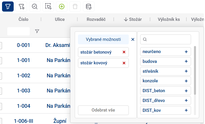
- **The Parcel Whisperer
The parcel whisperer contains two text fields that help you find specific parcels. The first one is used to enter the cadastral area, which can be done by word or code, both of which are assisted by the whisperer. The second field is used to enter specific parcel numbers.
There are two more help buttons below the text fields. The “Add records” option determines whether the newly searched parcel will be added to the end of the results table or whether older search results will be removed from the table.
“Group parcel search” allows the user to search for multiple parcel numbers at the same time.
- Spatial search
The spatial search works identically to the general search mode (General), the only modification is the option to “Add records” to Results Table.
Results table
6.1 RESULTS TABLE
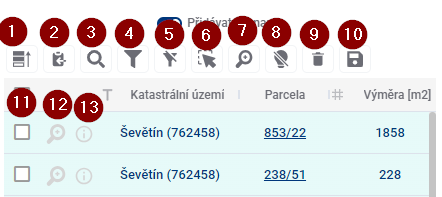
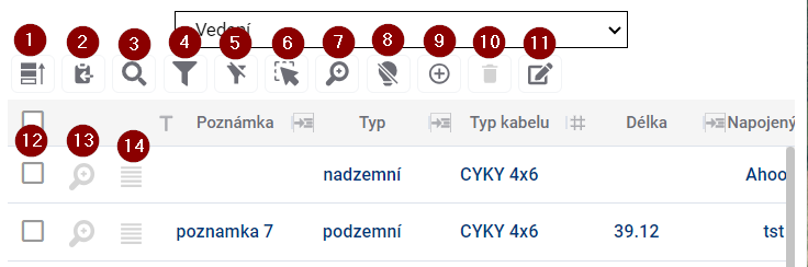
To control the results table, there is a group of tools above the table and another one directly in the table.
- Prioritize Selected - moves selected elements in the table before others
- Save selected to clipboard - and then you can paste the records into a text editor
- Search in data - a quick way to filter records using the text you enter
- Show/hide filter - show/hide text boxes to filter results for all columns
- Show only filtered in map - limits the visibility of features in the map to only those that are filtered
- Select elements in the map - allows to select and highlight a drawing by clicking in the map
- Browse to selected features - zooms to the selected features in the map window
- Disable highlighting of selected items
- Delete row - removes selected records from the results table. If none is selected, removes all of them.
- Export selected data - allows you to export the results table to a selected format, for example .xlsx
- Select item in table - click in the check box to select and highlight the record
- Browse to feature - zooms to the selected feature drawing in the map window
- Item information - opens detailed information about the item in the display panel
Select and highlight elements
When you hover over a row in the table, the row is highlighted and the drawing is highlighted in light blue in the map window.
Selected items are highlighted in dark blue in the table and in the map and can be selected either by checking the checkbox on the left side of the table or by clicking on the shape in the map window, but only with the Select items in map function (Button 6) enabled. Prioritize selected (Button 1) places the selected items at the top of the table.
Approaching the elements
Zooming the map to the elements can be achieved in two ways. Browse to selected elements (Button 7) zooms the map to the elements that are selected and therefore highlighted in the table, Browse to element (Button 12), located next to each record, zooms the map to that particular element.
Filtering elements
Element filtering allows you to display only those records in the results table whose attribute meets a certain condition. The easiest and fastest way to do this is to use the Search in Data tool (Button 3), which displays a text box to enter the desired constraint. Filters for all columns separately can be accessed using Show/Hide Filter (Button 4), and for each column you can still open a popup with a more detailed filter specification and change the operator from “equals” to “is greater than”, for example.
Element details
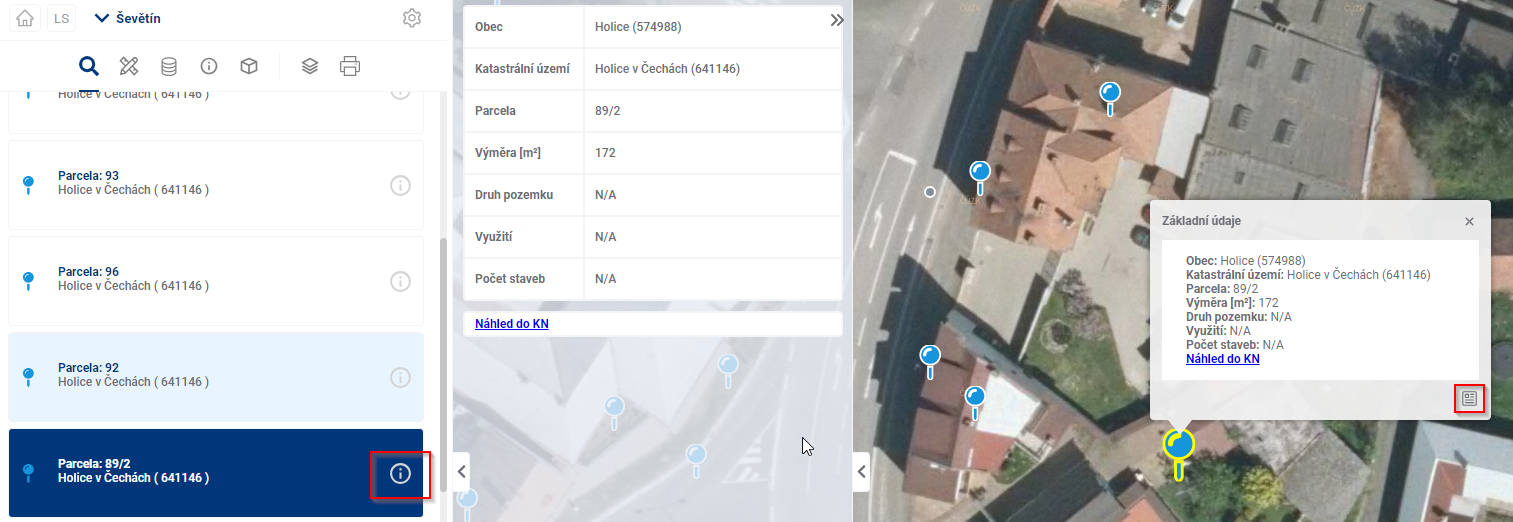
The details of the element can be displayed in the viewing panel by clicking on Information about the element (1) or on the button in the bottom right corner of the popup (2). From the viewing panel you can then use the blue link (3) to get to the Land Register Access website. This can also be done by clicking on the parcel number in the results table (4).

Data storage
Selected rows from the table can be saved to a file outside MGM in two different ways. A quicker and simpler solution can be achieved by using Save Selected to Clipboard (Button 2) and then pasting into, for example, an .xlsx file. The result then looks as follows:
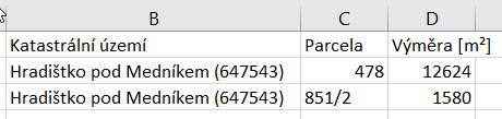
An alternative is Save rows (Button 10), which allows saving records again in the selected format - for example .xlsx or in a Shapefile file with geometry. The saved file has the current date in the name and contains more columns than saving to the clipboard. This spreadsheet data is identical to the parcel information displayed via popup or in the viewport.

Tabular data
7. TABULAR DATA
The tabular data module is the main place where customer data is stored and displayed. Utility data, passports, DTM data and more can be uploaded here. Data is displayed here in a clear table and also spatially in a map.
Adding new data to the project is done by the service administrator. You can easily switch between the data that are ready for the customer in the project in the drop-down menu in the work panel under the toolbar.
Working with the table
WORKING WITH TABLE
The table of records is prepared for the MawisGeodataManagement user so that he can work with it in the best and easiest way.
Layout and table size
The user can easily adjust the layout and size of the table by stretching the working panel (by dragging the panel edge - see chapter 1.1.GENERAL OPERATION OF THE APPLICATION) and also by stretching/narrowing the table columns themselves, or by rearranging the order of the table columns.
The width of the table column can be set by pressing the left mouse button and dragging the column border in the table header. Moving the column order can be done by pressing the left mouse button and dragging the column sideways.
The column width and column order settings are cached in the viewer, so they remain available even if you switch to another module (e.g. Layer Organizer) and come back.
Table and form
If the user is not comfortable working with the whole table, there is an option to switch the view to a form that displays only one element record, using the button on the left of the table.  One of the advantages of the form is that it can better display fields that contain text longer than one line.
If the value of the cell in the table is underlined, it means that the cell refers to a linked item in another table and it is possible to switch to the fomular of this linked item by Ctrl + click on the value (e.g. from the table Light places to the form of the connected Switchboard).
There are two ways to move between table cells:
- using the mouse - clicking on a cell will activate the cell selected by the user
- keyboard arrows - pressing the keyboard arrows moves the selected cell in the selected direction
You can use Ctrl + C to copy the displayed value from the selected cell to the clipboard and then paste it into Excel, email, etc.
Edit
Provided that the logged in user has the “Editor” role, and the table records are set as editable, it is possible to edit the records in the table. Double-clicking on a cell or pressing the “ENTER” key will activate the cell for editing (similar to MS Excel). Subsequently, the user can overwrite the contents of the table cell. The type of editing depends on the data type of the column. For example, for the data type “Date”, the user is offered to select a date from the calendar. For text fields, the user can directly type text and for numeric values, the options are offered in a drop-down box.
If longer text is inserted, the field is expanded and also added with a scroll bar on the side.
After editing, you need to confirm the change by pressing the “Enter” key or by simply clicking outside the edited cell. If the user tries to enter an unauthorized value into the cell, the cell will be highlighted in red. In this case, clicking outside the edited cell will return the record value to the original value.
The column data types are shown before the column name in the table header.
Select and highlight elements
When you hover the mouse over a row in the table, the row is highlighted and the item is highlighted in the map window. The same effect works when you move the mouse over an element in the map.
Working with files Assuming there is a file upload column in the table, files can be uploaded/downloaded/removed and viewed for each record in the table. Clicking on a file or double clicking in a field will open the File Gallery in the Display Panel and these operations can be performed there.
Simply clicking in the field in the table will open the File Browser, where you can again select a file to upload. The maximum file size is 20 Mb.
Table tools
TABLE SETTINGS
To control the table there is a group of tools above the table and another one directly in the table.
- Prioritize Selected - moves selected elements in the table before others
- Save selected to clipboard - and then you can paste the records into a text editor
- Search in data - a quick way to filter records using the text you enter
- Show/hide filter - show/hide text boxes to filter results for all columns
- Show only filtered in map - limits the visibility of features in the map to only those that are filtered
- Select map elements - allows you to select and highlight artwork by interacting with the map
- Browse to selected features - zooms to the selected features in the map window
- Disable highlighting of selected items
- Add new item - opens the form ready to add a new item
- Delete item - removes selected records from the results table
- Bulk data editing - allows to edit the column value for multiple items at the same time
- Select item in table - click in the check box to select and highlight the record
- Browse to feature - zooms to the selected feature drawing in the map window
- Open item form - opens the form for easier data editing
Select and highlight elements
When you hover over a row in the table, the row is highlighted and the drawing is highlighted in orange in the map window.
Selected features are also highlighted in the table and are yellow in the map and can be selected either by checking the checkbox on the left side of the table or by clicking on the shape in the map window, but only with the Select features in map function enabled (Button 6). You can use the polygon drawing to select multiple features. Clicking and dragging draws a rectangle, single clicks allow you to create a polygon of any shape. If the entire area of the map window is filled with the polygons in question, it is necessary to double click to start drawing the selection polygon. The drawing is terminated by double-clicking or right-clicking. Prioritize Selected (Button 1) places the selected elements at the top of the table.
Approaching the elements
Zooming the map to the elements can be achieved in two ways. Browse to selected elements (Button 7) zooms the map to the elements that are selected and therefore highlighted in the table, Browse to element (Button 12), located next to each record, zooms the map to that particular element. The same button is also available in the element form.
Filtering elements
Element filtering allows you to display only those records in the results table whose attribute meets a certain condition. The easiest and fastest way to do this is to use the Search in Data tool (Button 3), which displays a text box to enter the desired constraint. Filters for all columns separately can be accessed using Show/Hide Filter (Button 4), and for each column you can still open a popup with a more detailed filter specification and change the operator from “equals” to “is greater than”, for example. In the case of filtering in a dial column, it is possible to select directly from existing values.
Data storage
Selected rows from the table can be saved to a file outside the geoportal using Save selected to clipboard (Button 2) and then pasted into, for example, an .xlsx file.
Adding a new item
The add new item button (Button 9) redirects to the empty new item form and starts drawing in the map.
- To add a point to the map, simply click anywhere in the map window
- The line drawing is done in such a way that each click adds a new breakpoint to the element, then double-clicking ends the drawing of the element together with the creation of the point. A right click will also end the drawing, but at the previous point.
- polygon drawing, you can add closed broken lines to the map. Drawing is done by each click adding a new refraction point to the element, then double-clicking to close the polygon by connecting the click point to the origin and ending the drawing of the element. A right click also ends the drawing, but without creating a new point at the click point.
After drawing the item it is possible to fill in attributes and with the corresponding buttons to confirm or discard the currently created item and return to the table view
In the drop-down menu in the form it is also possible to turn on/off the snapping to existing map features when drawing
Working with elements in the map
WORKING WITH MAP FEATURES
Data with spatial information is displayed in the map window. Whether the elements are currently displayed in the map can be set in the Layer Organizer.
Hovering over an item in the map will highlight the item in the map (the symbol will be enlarged or highlighted in colour) and also highlight the corresponding record in the table (in light blue).
Simply click on an item in the map to display basic information in the pop-up menu above the item. Double-click on an element in the map to see detailed information about the element in the form in the taskbar.
Geometry editing
EDITATION GEOMETRY
Editing the position of registered elements is available via the form of the specific element.
Click and drag a point on the map to edit the item. Vertices of lines and polygons can be added by clicking on an edge and removed by clicking and pressing the CTRL key.
It is possible to set whether the edited points should be attached to other vector layers or not.
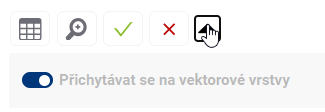
At the end, the editing must be confirmed or discarded with the appropriate buttons  .
.
Taskmanager
8th module TASKMANAGER
The Taskmanager module extends the functionality of the notes from the Measurement module with a complex workflow and notification system. It is used to manage a data layer with tasks that have their location and can be assigned to other application users and record their status. The data is displayed here in a clear table and also spatially in a map. Tasks can be assigned to all users involved in the project. The task manager is also set up so that only tasks that have been assigned to a user or that the user has entered can be edited. The tasks of other users can be viewed and possibly commented on.
Overview of tasks
View tasks
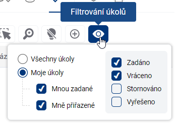
In addition to the name, each task also has its Assignor (the user who created it), Solver (the assigned user who is to complete the task), status, and date of creation. Tasks in the table can be filtered by the affiliation to the logged-in user and by status, in addition to the common tools in chapter 10.2 TABLE TOOLS.
- The default view shows:
- Tasks entered by the user (the logged-in user is the Task Assignor)
- Tasks assigned to the user (the logged-in user is the Task Solver)
- The “Eye” button allows you to switch between:
- Personal tasks
- All tasks in the system
- Displayed task statuses (entered, solved, returned, cancelled, archived)
Task states
Each task is visually marked on the map with a marker with a colored dot indicating its current status:
- Orange: task completed
- Red: Task returned
- Green: task solved
- Yellow: task cancelled
- Grey: Task archived
Task management
Creating a task
- In the task table, click on “Add new task”
- Select the task location on the map
- Various map layers are available:
- Real estate cadastre
- Municipal address points
- Specialized administrator layers
- Various map layers are available:
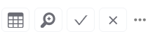
Saving changes
- All changes to the task must be confirmed and saved:
- To save changes, click on the checkmark icon labeled “Save Changes”
- To discard changes, use the x icon with the label “Discard changes”
- This applies in particular to:
- Assigning the task to a new solver
- Changes to task status
- Editing information in a task
- Changes to the location of a task on the map
Task assignment
- You can assign a task to any user in the system
- Automatic email notifications are sent after changes are assigned and saved:
- To the contracting authority
- To the new researcher
Editing a task
- Only:
- Task sponsor
- Current assigned solver
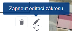
- Change the position of the task:
- Click the pencil icon to activate location editing
- Move a point to a new position on the map
- Don’t forget to confirm the change by saving
- All changes must be confirmed by saving
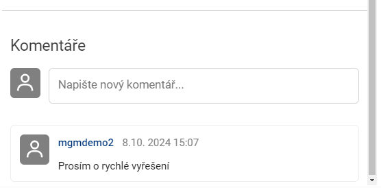
Comments
When you open the task detail form, there is a comments section at the bottom where interested users can exchange messages about the task. New comments, as well as other changes to the status of the task, are notified to users by email notifications.
- Anyone with permission to see the task can comment on the task
- Additional information can be added to the task
Workflow of tasks
Status change procedure
- Entered (red)
- Resolved (green)
- Returned (original red)
- Canceled (yellow)
- Archived (grey)
- Each change of status must be confirmed by saving
Notification
- Each saved task status change is accompanied by an email notification
- Email notifications contain a link directly to a specific task in the system
- Notifications are not sent to the user who immediately made the change. They are always sent to the “others”.
Mobile access
Functionality on a mobile device
- Viewing and managing tasks is partially functional on mobile devices
Working with the table
WORKING WITH TABLE
The table of records is prepared for the MawisGeodataManagement user so that he can work with it in the best and easiest way.
Layout and table size
The user can easily adjust the layout and size of the table by stretching the working panel (by dragging the panel edge - see chapter 1.1.GENERAL OPERATION OF THE APPLICATION) and also by stretching/narrowing the table columns themselves, or by rearranging the order of the table columns.
The width of the table column can be set by pressing the left mouse button and dragging the column border in the table header. Moving the column order can be done by pressing the left mouse button and dragging the column sideways.
The column width and column order settings are cached in the viewer, so they remain available even if you switch to another module (e.g. Layer Organizer) and come back.
Table and form
If the user is not comfortable working with the whole table, there is an option to switch the view to a form that displays only one element record, using the button on the left of the table. One of the advantages of the form is that it can better display fields that contain text longer than one line.
If the value of the cell in the table is underlined, it means that the cell refers to a linked item in another table and it is possible to switch to the fomular of this linked item by Ctrl + click on the value (e.g. from the table Light places to the form of the connected Switchboard).
There are two ways to move between table cells:
- using the mouse - clicking on a cell will activate the cell selected by the user
- keyboard arrows - pressing the keyboard arrows moves the selected cell in the selected direction
You can use Ctrl + C to copy the displayed value from the selected cell to the clipboard and then paste it into Excel, email, etc.
Edit
Provided that the logged in user has the “Editor” role, and the table records are set as editable, it is possible to edit the records in the table. Double-clicking on a cell or pressing the “ENTER” key will activate the cell for editing (similar to MS Excel). Subsequently, the user can overwrite the contents of the table cell. The type of editing depends on the data type of the column. For example, for the data type “Date”, the user is offered to select a date from the calendar. For text fields, the user can directly type text and for numeric values, the options are offered in a drop-down box.
If longer text is inserted, the field is expanded and also added with a scroll bar on the side.
After editing, you need to confirm the change by pressing the “Enter” key or by simply clicking outside the edited cell. If the user tries to enter an unauthorized value into the cell, the cell will be highlighted in red. In this case, clicking outside the edited cell will return the record value to the original value.
The column data types are shown before the column name in the table header.
Select and highlight elements
When you hover the mouse over a row in the table, the row is highlighted and the item is highlighted in the map window. The same effect works when you move the mouse over an element in the map.
Working with files Assuming there is a file upload column in the table, files can be uploaded/downloaded/removed and viewed for each record in the table. Clicking on a file or double clicking in a field will open the File Gallery in the Display Panel and these operations can be performed there.
Simply clicking in the field in the table will open the File Browser, where you can again select a file to upload. The maximum file size is 20 Mb.
Table tools
TABLE SETTINGS
To control the table there is a group of tools above the table and another one directly in the table.
- Prioritize Selected - moves selected elements in the table before others
- Save selected to clipboard - and then you can paste the records into a text editor
- Search in data - a quick way to filter records using the text you enter
- Show/hide filter - show/hide text boxes to filter results for all columns
- Show only filtered in map - limits the visibility of features in the map to only those that are filtered
- Select map elements - allows you to select and highlight artwork by interacting with the map
- Browse to selected features - zooms to the selected features in the map window
- Disable highlighting of selected items
- Add new item - opens the form ready to add a new item
- Delete item - removes selected records from the results table
- Bulk data editing - allows to edit the column value for multiple items at the same time
- Select item in table - click in the check box to select and highlight the record
- Browse to feature - zooms to the selected feature drawing in the map window
- Open item form - opens the form for easier data editing
Select and highlight elements
When you hover over a row in the table, the row is highlighted and the drawing is highlighted in orange in the map window.
Selected features are also highlighted in the table and are yellow in the map and can be selected either by checking the checkbox on the left side of the table or by clicking on the shape in the map window, but only with the Select features in map function enabled (Button 6). You can use the polygon drawing to select multiple features. Clicking and dragging draws a rectangle, single clicks allow you to create a polygon of any shape. If the entire area of the map window is filled with the polygons in question, it is necessary to double click to start drawing the selection polygon. The drawing is terminated by double-clicking or right-clicking. Prioritize Selected (Button 1) places the selected elements at the top of the table.
Approaching the elements
Zooming the map to the elements can be achieved in two ways. Browse to selected elements (Button 7) zooms the map to the elements that are selected and therefore highlighted in the table, Browse to element (Button 12), located next to each record, zooms the map to that particular element. The same button is also available in the element form.
Filtering elements
Element filtering allows you to display only those records in the results table whose attribute meets a certain condition. The easiest and fastest way to do this is to use the Search in Data tool (Button 3), which displays a text box to enter the desired constraint. Filters for all columns separately can be accessed using Show/Hide Filter (Button 4), and for each column you can still open a popup with a more detailed filter specification and change the operator from “equals” to “is greater than”, for example. In the case of filtering in a dial column, it is possible to select directly from existing values.
Data storage
Selected rows from the table can be saved to a file outside the geoportal using Save selected to clipboard (Button 2) and then pasted into, for example, an .xlsx file.
Adding a new item
The add new item button (Button 9) redirects to the empty new item form and starts drawing in the map.
- To add a point to the map, simply click anywhere in the map window
- The line drawing is done in such a way that each click adds a new breakpoint to the element, then double-clicking ends the drawing of the element together with the creation of the point. A right click will also end the drawing, but at the previous point.
- polygon drawing, you can add closed broken lines to the map. Drawing is done by each click adding a new refraction point to the element, then double-clicking to close the polygon by connecting the click point to the origin and ending the drawing of the element. A right click also ends the drawing, but without creating a new point at the click point.
After drawing the item it is possible to fill in attributes and with the corresponding buttons to confirm or discard the currently created item and return to the table view
In the drop-down menu in the form it is also possible to turn on/off the snapping to existing map features when drawing
Working with elements in the map
WORKING WITH MAP FEATURES
Data with spatial information is displayed in the map window. Whether the elements are currently displayed in the map can be set in the Layer Organizer.
Hovering over an item in the map will highlight the item in the map (the symbol will be enlarged or highlighted in colour) and also highlight the corresponding record in the table (in light blue).
Simply click on an item in the map to display basic information in the pop-up menu above the item. Double-click on an element in the map to see detailed information about the element in the form in the taskbar.
Geometry editing
EDITATION GEOMETRY
Editing the position of registered elements is available via the form of the specific element.
Click and drag a point on the map to edit the item. Vertices of lines and polygons can be added by clicking on an edge and removed by clicking and pressing the CTRL key.
It is possible to set whether the edited points should be attached to other vector layers or not.
At the end, the editing must be confirmed or discarded with the appropriate buttons .
3D Models
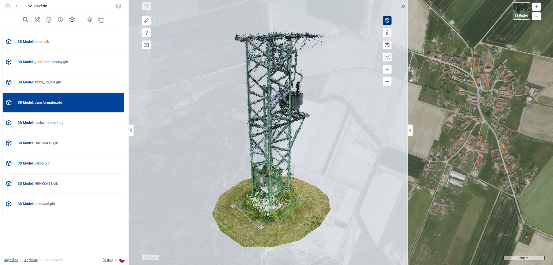
9. 3D MODELS
In the 3D Models module you can operate all available 3D models within the project.
only the administrator can add 3D models to the project.
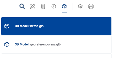
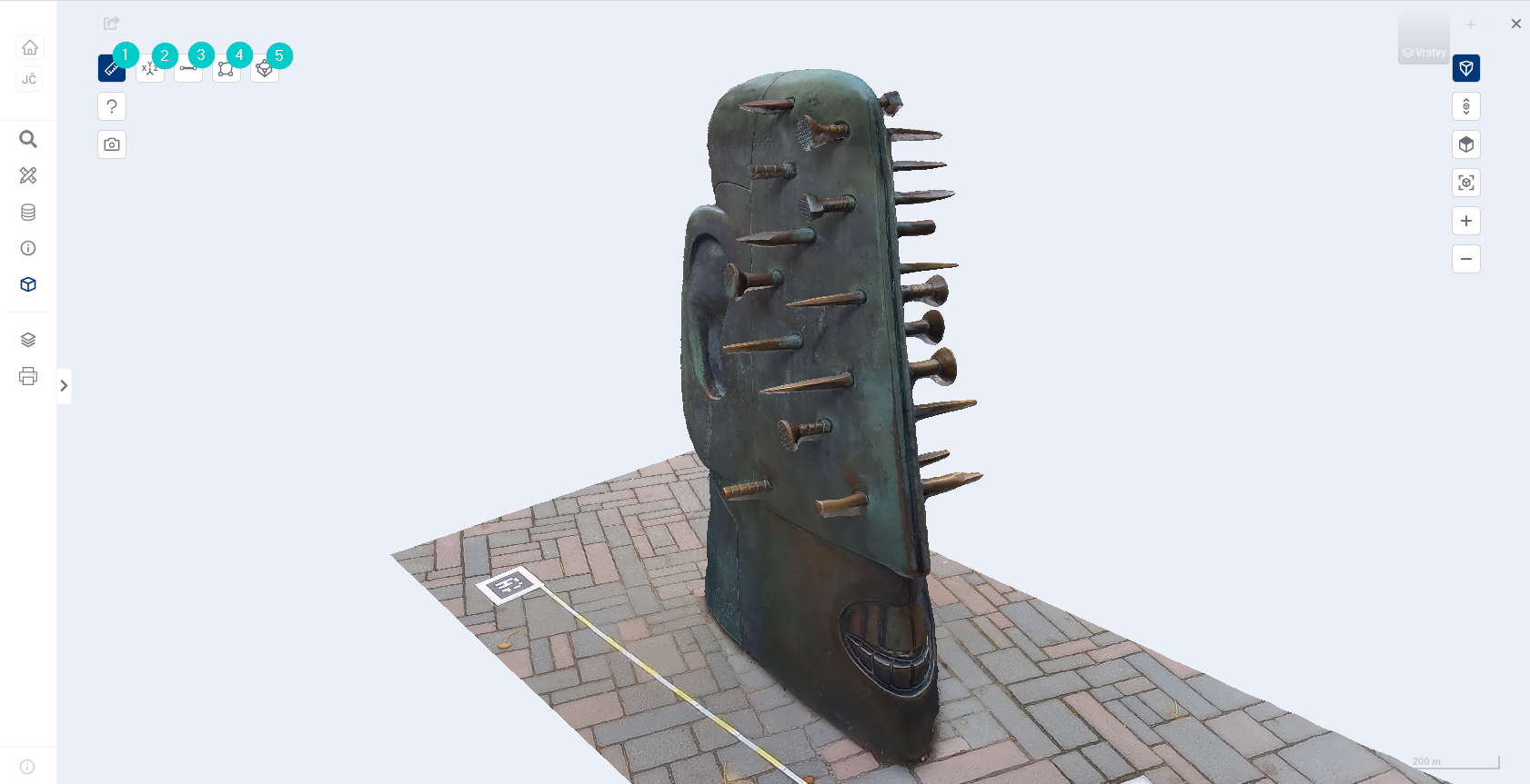
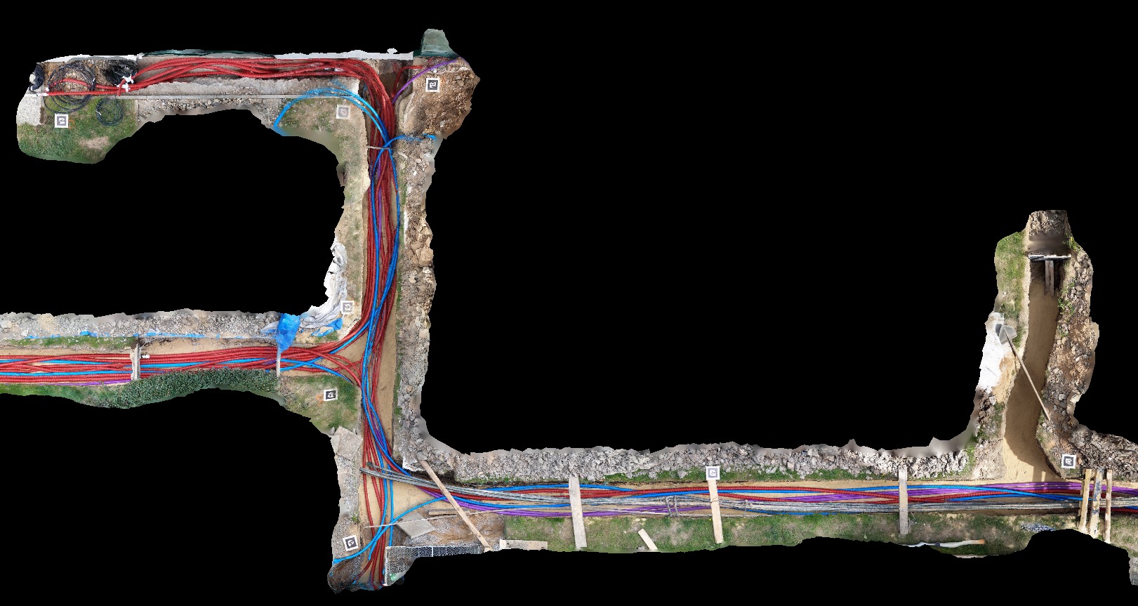
The user selects a 3D model to display from the list in the main panel. The 3D viewer environment is then launched in the display panel and the selected 3D model is loaded.
3D space control
9.1. 3D-space control
Movement in the 3D space of the browser can be done with the mouse, keyboard and specialised functions. The use of these functions is independent of the measurement functions and can be used simultaneously without interrupting the measurement.
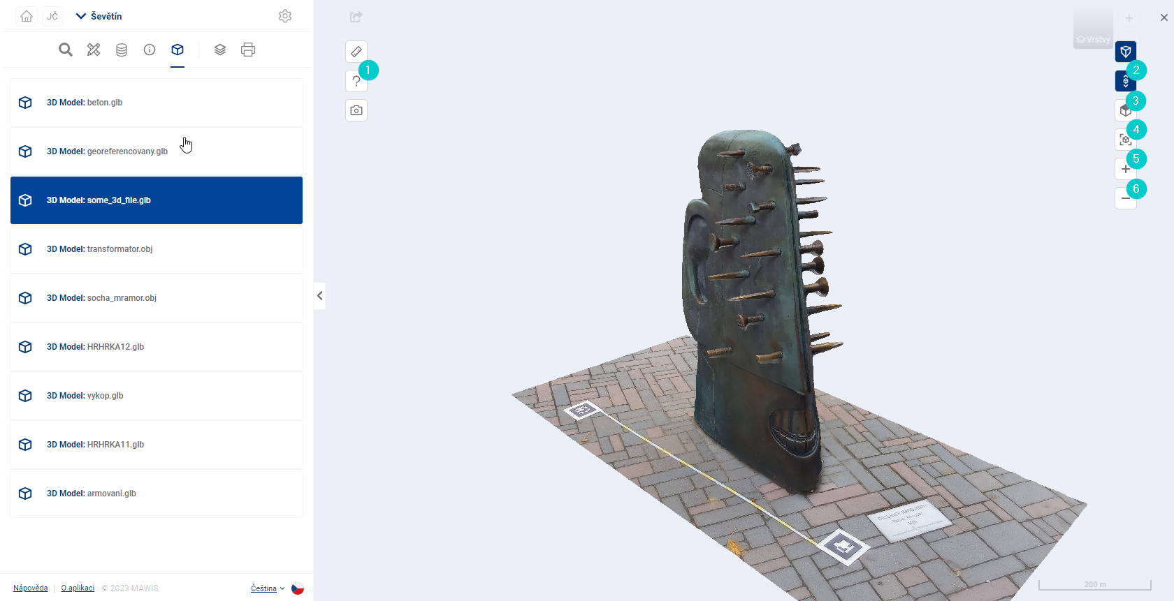
- Help - a guide describing operations that affect the 3D model display.
- Vertical Scroll - switches the navigation mode in 3D space to allow the 3D model to be scrolled vertically.
- Top view - rotates the 3D model to top view, with the projection axis parallel to the Z axis.
- Default view - returns the 3D model to the same view as after loading. The model will be displayed in its entirety from the oblique ISO view.
- Zoom - zooms in on the 3D model.
- Delay - delays the 3D model.
FAVOR
The model can be moved in 3D space using the cursor keys or by grabbing the model with the right mouse button and moving the mouse.

In the default mode, the model shifts in the horizontal plane. This mode is suitable for horizontally oriented 3D models, such as excavations.
Alternatively, Vertical Shift (#6 above) can be activated to shift the plane in which the 3D space is rotated. This mode is suitable for vertically oriented 3D models, such as sculptures.

ZOOM
The model can be zoomed in or out with the mouse wheel, by pressing the wheel and moving the mouse, or by using the  and
and  buttons.

ROTATION
The model can be rotated by holding down the right mouse button and moving the mouse.

OTHER NAVIGATION FUNCTIONS
Demonstration of Hint, Top View and Default View:
Measuring and plotting points
9.2. MEASUREMENT AND EXTRACTION OF POINTS
the 3D viewer allows you to plot points in the model, find their coordinates or measure distances, areas and volumes.
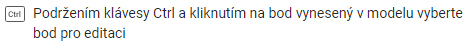
The method of entering, editing and deleting points is common to all measurement functions.
MEASUREMENT FUNCTION
- Display menu of measurement functions
- Coordinates
- Distance
- Area
- Volume
It is not possible to use different measurement functions at the same time or to plot and display elements of different measurement functions at the same time. The user is warned by the system of the possible loss of entered data when the measurement is terminated or the measurement function is switched.
POINT DEDUCTION

EDITING POINT
REMOVING A POINT
Any point can be removed by clicking on  in the point table.
Coordinates
9.2.1 SOUŘADNICE

The user can use the Coordinates tool to enter points at arbitrary locations on the model surface. The system automatically prints the [X, Y, Z] coordinates of the point. The user can write annotations to the points and export them to a file.
The plotting of points is described in detail in the parent chapter 9.2.
NOTE ON POINT
It is possible to write notes with a maximum length of 15 characters for the recorded points.
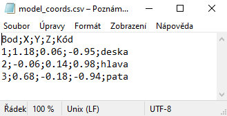
EXPORT COORDINATES
The export allows the user to download a CSV file that contains all the points and their data, including a note. The downloaded file contains a header.
_Note: for correct loading of CSV into MS Excel it is necessary to use the import tool “Z Text/CSV” on the Data tab
Distance
9.2.2. VZDÁLENOST

Distance measurement allows you to calculate the length of the line of two or more user entered points and some other values based on them. A distinction is made between data calculated for individual points and aggregated measurement results.
The plotting of points is described in detail in the parent chapter 9.2.
The distance measurement uses all the coordinate measurement functions listed in chapter 9.2.1.
The export of coordinates and measurement results is described in chapter 9.3.
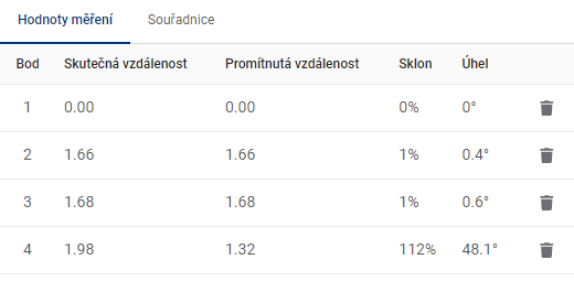
MEASUREMENT VALUES
The table Measurement values shows the calculations for each measurement point.
-
Actual distance = the distance corresponding to the link between this point and the previous point. In the case of the first point, the value 0 is given.
-
Projected distance = the distance corresponding to the length of the horizontal overhang (with angle 0°) in an imaginary triangle, where this point represents the vertex between the overhang and the horizontal overhang. The previous point then represents the vertex between the hypotenuse and the vertical suspension (with an angle of 90°). In the case of the first point the value 0 is given.
-
Slope = standard calculation of the slope of the line joining this point and the previous point, given in whole percent.
-
Angle = the angle between the line (this point - previous point) and the horizontal plane, given in degrees.
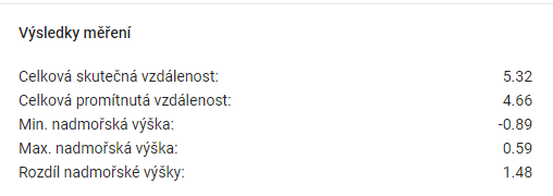
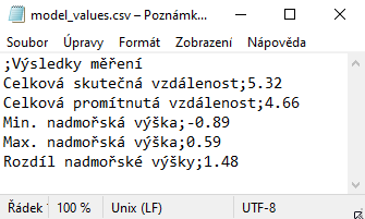
MEASUREMENT RESULTS
The Measurement Results table shows the summary data calculated for the measurements.
-
Total Actual Distance = the sum of all Actual Distances from the Measurement Values table.
-
Total Projected Distance = the sum of all Projected Distances from the Measurement Values table.
-
Min. altitude = the point with the lowest coordinate value on the Z axis.
-
Max altitude = the point with the highest coordinate value on the Z axis.
-
Difference in altitude = difference between Max. altitude difference between Min. and Min. altitude.
Area
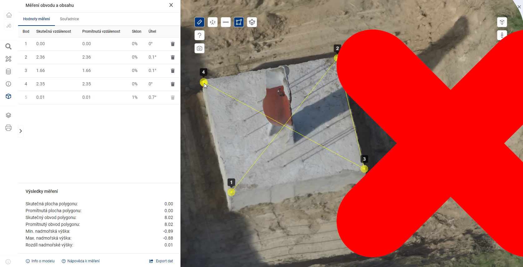
9.2.3. PLOCHA

The user can mark three or more points in the model representing the vertices of a 3D polygon, to which the perimeter and area are immediately calculated. Similar to distance measurements, data is calculated for individual points and the entire area.
The plotting of points is described in detail in the parent chapter 9.2.
The area measurement uses the coordinate measurement function 9.2.1 and the distance measurement function 9.2.2.
The export of coordinates and measurement results is described in chapter 9.3.
The area of the polygon cannot be calculated and closed if there is a line crossing.
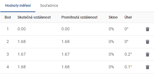
MEASUREMENT VALUES
The table Measurement values shows the calculations for each measurement point.
-
Actual distance = the distance corresponding to the link between this point and the previous point. In the case of the first point, the value 0 is given.
-
Projected distance = the distance corresponding to the length of the horizontal overhang (with angle 0°) in an imaginary triangle, where this point represents the vertex between the overhang and the horizontal overhang. The previous point then represents the vertex between the hypotenuse and the vertical suspension (with an angle of 90°). In the case of the first point the value 0 is given.
-
Slope = standard calculation of the slope of the line joining this point and the previous point, given in whole percent.
-
Angle = the angle between the line (this point - previous point) and the horizontal plane, given in degrees.
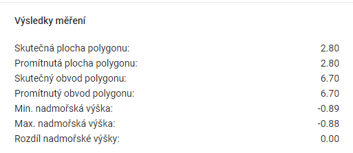
MEASUREMENT RESULTS
The Measurement Results table shows the summary data calculated for the measurements.
-
Real polygon area = polygon area in 3D space.
-
Projected polygon area = the area of a 2D polygon that is the orthogonal projection of a 3D polygon onto a horizontal surface.
-
Real polygon perimeter = the sum of the lengths of all sides of the polygon in 3D space.
-
Projected polygon perimeter = the perimeter of a 2D polygon that is the orthogonal projection of a 3D polygon onto a horizontal surface.
-
Min. altitude = the point with the lowest coordinate value on the Z axis.
-
Max altitude = the point with the highest coordinate value on the Z axis.
-
Difference in altitude = difference between Max. altitude difference between Min. and Min. altitude.
Volume
9.2.4. OBJEM

The tool automatically calculates the volume in a user-defined part of the model. In the first steps, the control of the tool is similar to area measurement. The user places points in the model, which are immediately triangulated into a reference 3D surface. The perimeter of the reference surface must not cross itself or the edge of the model.
After the right-clicking of the points, the volume calculation is performed. It is symbolized by an animation in the model and takes a few seconds. The volume of the space between the reference surface and the model surface is measured. The calculation is 2.5D, that is, if there are multiple collisions with the surface at any location [X,Y], only the location with the smallest Z coordinate is considered for the calculation. For example, overhangs or pipes running above ground are ignored. During the calculation, the space is imaginary filled with small blocks. The result is the sum of their volumes. The spaces below the reference surface (excavation) and above it (excavation) are shown separately in the results.
The plotting of points is described in detail in the parent chapter 9.2.
The volume measurement uses the coordinate measurement function 9.2.1, distance 9.2.2 and area 9.2.3.
The export of coordinates and measurement results is described in chapter 9.3.
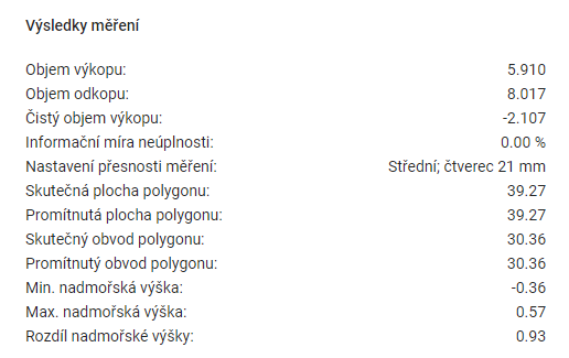
MEASUREMENT RESULTS
The Measurement Results table shows the summary data calculated for the measurements.
-
Excavation volume = the volume of the 3D model above the reference surface.
-
Dig volume = the volume of the 3D model under the reference surface.
-
Clean excavation volume = excavation volume minus the excavation volume.
-
Information Incompleteness Rate = percentage of surface area for which the volume could not be calculated. It is greater than 0 only at the location of a defect (“hole”) in the 3D model.
-
Measurement accuracy setting = the size of the grid used to measure the volume.
-
Real polygon area = polygon area in 3D space.
-
Projected polygon area = the area of a 2D polygon that is the orthogonal projection of a 3D polygon onto a horizontal surface.
-
Real polygon perimeter = the sum of the lengths of all sides of the polygon in 3D space.
-
Projected polygon perimeter = the perimeter of a 2D polygon that is the orthogonal projection of a 3D polygon onto a horizontal surface.
-
Min. altitude = the point with the lowest coordinate value on the Z axis.
-
Max altitude = the point with the highest coordinate value on the Z axis.
-
Difference in altitude = difference between Max. altitude difference between Min. and Min. altitude.
MEASUREMENT SETTINGS
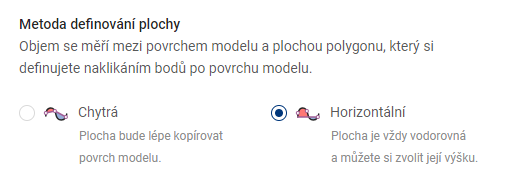
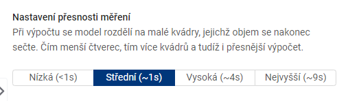
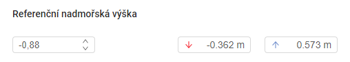
The reference altitude is used to set the height of the plane in the case of measurements by the Horizontal method.
MEASUREMENT VALUES
The table Measurement values shows the calculations for each measurement point.
-
Actual distance = the distance corresponding to the link between this point and the previous point. In the case of the first point, the value 0 is given.
-
Projected distance = the distance corresponding to the length of the horizontal overhang (with angle 0°) in an imaginary triangle, where this point represents the vertex between the overhang and the horizontal overhang. The preceding point then represents the vertex between the hypotenuse and the vertical suspension (with an angle of 90°). In the case of the first point the value 0 is given.
Other 3D viewer features
9.3. OTHER FUNCTIONS OF THE 3D VIEWER
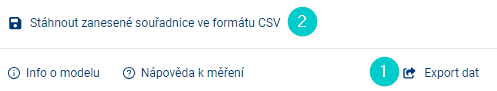
EXPORT DAT
In the foot of the measurement panel, you can download the CSV file with the coordinates of the recorded points or the log with the measurement results (2) via the menu Data export (1).
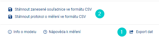
the Coordinate Export prepares a file in CSV format for the user, which contains all the entered points and their data, including a note. The downloaded file contains a header.
Export results downloads a file in CSV format that contains all the results of the measurement.
_Note: for correct loading of CSV into MS Excel it is necessary to use the import tool “Z Text/CSV” on the Data tab
IMAGE OF MODEL

The Off/Off Perspective function changes the way differently spaced parts of the model are rendered.
-
Perspective type of view
The default setting is always a perspective type of view. This allows for a 3D model that is close to human vision, but distorts the angles.
-
** Orthographic view type**
The user can switch the perspective type of the camera to the orthographic (perspective off) view type at any time. This allows more accurate placement of points in the 3D model and facilitates some measurement functions. Under this view type, perspective is ignored and the 3D model is not rendered faithfully.
The combination of Perspective Off and Top View will display the 3D model just like an orthophoto.
SCREEN SHOT

This function saves the current view of the 3D model as an image in JPG format.
Support for expression
10. SUPPORT FOR EXPRESSION
The module support for comments is used by technical infrastructure managers who have a legal obligation to comment on requests for the existence of networks. This module assists administrators with the agenda of commenting on the existence of networks.
The administrator has a register of requests to be commented on in the module. Each row in the table represents one request.
- The applications are in one clear table
- The outline of the area of interest of each application is shown on a map
- Automatically move requests from MawisUtility
- You can add and plot your own request (for example, one that has been emailed or mailed to the administrator) to the table
- The administrator can record the status of a request, i.e. whether the request has already been processed
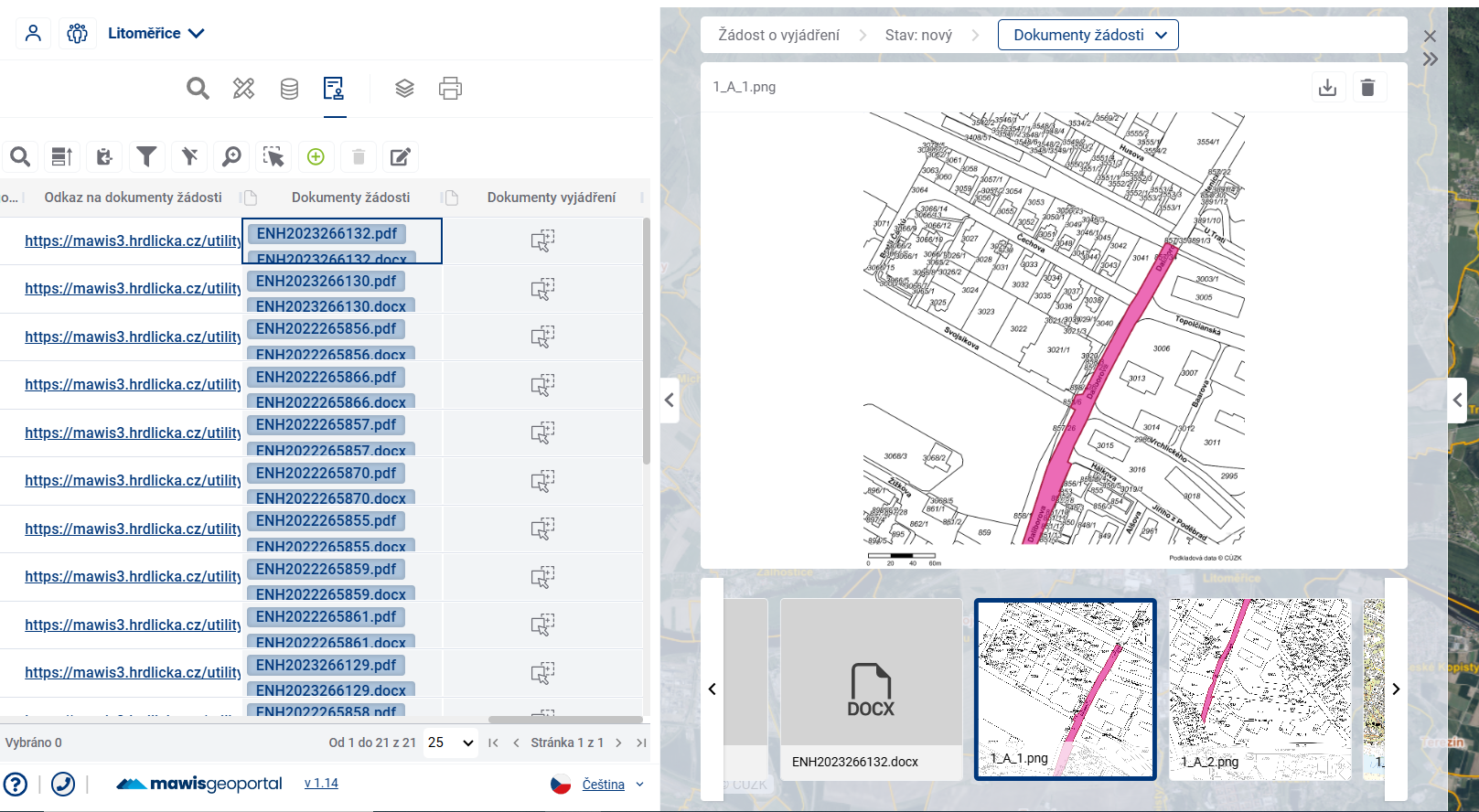
- The administrator has the ability to view and download attachments to the application (PDF of the application, drawing image, attachments to the application and more … )
- The application can be uploaded with documents of representation
- Representation documents can be sent to the applicant with one button
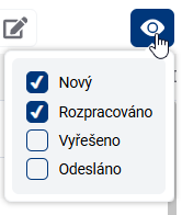
by default, the Expression Support table displays requests that have not yet been processed by the administrator (do not have a status of “Resolved” and “Sent”). The displayed requests can be filtered by the “eye” tool on the right above the table according to the processing status.
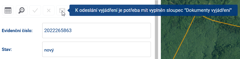
The “Representation Documents “ column is used to upload a representation to the application. This will allow the administrator to record a representation on one record of the request. In the request detail (form) , the administrator then has the option to send the uploaded representation documents to the requester. The statement can only be sent if there is an attachment uploaded in the “Statement Documents” column.
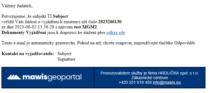
After pressing the “Send Statement “ button, a notification with a download link will be sent to the applicant’s email address by the administrator of the prepared withdrawal documents. The application is also automatically set to the “Submitted “ status. Sample notification:
The TI administrator can also have their network data uploaded to the application so they can easily visually see if requests are conflicting with the infrastructure they manage. The columns of the Expression Agenda table are administratively configurable - you can set what attributes are displayed in the table.
Working with the table
WORKING WITH TABLE
The table of records is prepared for the MawisGeodataManagement user so that he can work with it in the best and easiest way.
Layout and table size
The user can easily adjust the layout and size of the table by stretching the working panel (by dragging the panel edge - see chapter 1.1.GENERAL OPERATION OF THE APPLICATION) and also by stretching/narrowing the table columns themselves, or by rearranging the order of the table columns.
The width of the table column can be set by pressing the left mouse button and dragging the column border in the table header. Moving the column order can be done by pressing the left mouse button and dragging the column sideways.
The column width and column order settings are cached in the viewer, so they remain available even if you switch to another module (e.g. Layer Organizer) and come back.
Table and form
If the user is not comfortable working with the whole table, there is an option to switch the view to a form that displays only one element record, using the button on the left of the table. One of the advantages of the form is that it can better display fields that contain text longer than one line.
If the value of the cell in the table is underlined, it means that the cell refers to a linked item in another table and it is possible to switch to the fomular of this linked item by Ctrl + click on the value (e.g. from the table Light places to the form of the connected Switchboard).
There are two ways to move between table cells:
- using the mouse - clicking on a cell will activate the cell selected by the user
- keyboard arrows - pressing the keyboard arrows moves the selected cell in the selected direction
You can use Ctrl + C to copy the displayed value from the selected cell to the clipboard and then paste it into Excel, email, etc.
Edit
Provided that the logged in user has the “Editor” role, and the table records are set as editable, it is possible to edit the records in the table. Double-clicking on a cell or pressing the “ENTER” key will activate the cell for editing (similar to MS Excel). Subsequently, the user can overwrite the contents of the table cell. The type of editing depends on the data type of the column. For example, for the data type “Date”, the user is offered to select a date from the calendar. For text fields, the user can directly type text and for numeric values, the options are offered in a drop-down box.
If longer text is inserted, the field is expanded and also added with a scroll bar on the side.
After editing, you need to confirm the change by pressing the “Enter” key or by simply clicking outside the edited cell. If the user tries to enter an unauthorized value into the cell, the cell will be highlighted in red. In this case, clicking outside the edited cell will return the record value to the original value.
The column data types are shown before the column name in the table header.
Select and highlight elements
When you hover the mouse over a row in the table, the row is highlighted and the item is highlighted in the map window. The same effect works when you move the mouse over an element in the map.
Working with files Assuming there is a file upload column in the table, files can be uploaded/downloaded/removed and viewed for each record in the table. Clicking on a file or double clicking in a field will open the File Gallery in the Display Panel and these operations can be performed there.
Simply clicking in the field in the table will open the File Browser, where you can again select a file to upload. The maximum file size is 20 Mb.
Table tools
TABLE SETTINGS
To control the table there is a group of tools above the table and another one directly in the table.
- Prioritize Selected - moves selected elements in the table before others
- Save selected to clipboard - and then you can paste the records into a text editor
- Search in data - a quick way to filter records using the text you enter
- Show/hide filter - show/hide text boxes to filter results for all columns
- Show only filtered in map - limits the visibility of features in the map to only those that are filtered
- Select map elements - allows you to select and highlight artwork by interacting with the map
- Browse to selected features - zooms to the selected features in the map window
- Disable highlighting of selected items
- Add new item - opens the form ready to add a new item
- Delete item - removes selected records from the results table
- Bulk data editing - allows to edit the column value for multiple items at the same time
- Select item in table - click in the check box to select and highlight the record
- Browse to feature - zooms to the selected feature drawing in the map window
- Open item form - opens the form for easier data editing
Select and highlight elements
When you hover over a row in the table, the row is highlighted and the drawing is highlighted in orange in the map window.
Selected features are also highlighted in the table and are yellow in the map and can be selected either by checking the checkbox on the left side of the table or by clicking on the shape in the map window, but only with the Select features in map function enabled (Button 6). You can use the polygon drawing to select multiple features. Clicking and dragging draws a rectangle, single clicks allow you to create a polygon of any shape. If the entire area of the map window is filled with the polygons in question, it is necessary to double click to start drawing the selection polygon. The drawing is terminated by double-clicking or right-clicking. Prioritize Selected (Button 1) places the selected elements at the top of the table.
Approaching the elements
Zooming the map to the elements can be achieved in two ways. Browse to selected elements (Button 7) zooms the map to the elements that are selected and therefore highlighted in the table, Browse to element (Button 12), located next to each record, zooms the map to that particular element. The same button is also available in the element form.
Filtering elements
Element filtering allows you to display only those records in the results table whose attribute meets a certain condition. The easiest and fastest way to do this is to use the Search in Data tool (Button 3), which displays a text box to enter the desired constraint. Filters for all columns separately can be accessed using Show/Hide Filter (Button 4), and for each column you can still open a popup with a more detailed filter specification and change the operator from “equals” to “is greater than”, for example. In the case of filtering in a dial column, it is possible to select directly from existing values.
Data storage
Selected rows from the table can be saved to a file outside the geoportal using Save selected to clipboard (Button 2) and then pasted into, for example, an .xlsx file.
Adding a new item
The add new item button (Button 9) redirects to the empty new item form and starts drawing in the map.
- To add a point to the map, simply click anywhere in the map window
- The line drawing is done in such a way that each click adds a new breakpoint to the element, then double-clicking ends the drawing of the element together with the creation of the point. A right click will also end the drawing, but at the previous point.
- polygon drawing, you can add closed broken lines to the map. Drawing is done by each click adding a new refraction point to the element, then double-clicking to close the polygon by connecting the click point to the origin and ending the drawing of the element. A right click also ends the drawing, but without creating a new point at the click point.
After drawing the item it is possible to fill in attributes and with the corresponding buttons to confirm or discard the currently created item and return to the table view
In the drop-down menu in the form it is also possible to turn on/off the snapping to existing map features when drawing
Working with elements in the map
WORKING WITH MAP FEATURES
Data with spatial information is displayed in the map window. Whether the elements are currently displayed in the map can be set in the Layer Organizer.
Hovering over an item in the map will highlight the item in the map (the symbol will be enlarged or highlighted in colour) and also highlight the corresponding record in the table (in light blue).
Simply click on an item in the map to display basic information in the pop-up menu above the item. Double-click on an element in the map to see detailed information about the element in the form in the taskbar.
Geometry editing
EDITATION GEOMETRY
Editing the position of registered elements is available via the form of the specific element.
Click and drag a point on the map to edit the item. Vertices of lines and polygons can be added by clicking on an edge and removed by clicking and pressing the CTRL key.
It is possible to set whether the edited points should be attached to other vector layers or not.
At the end, the editing must be confirmed or discarded with the appropriate buttons .
Videos MawisGeoportal
11. VIDEONÁVODY
Promo videos introducing the MAWIS Geoportal product can be found at https://mawis.eu/videa/
Webinar recording November 2024 Autumn News: https://youtu.be/GEgAeUy6iyY
Introductory overview of displayed layers
The video explains the basic division of map layers in MawisGeoportal and shows how to navigate through them. The user will learn how to recognize project data, user layers and base maps and understand how the different groups work together to display information about an area. The tutorial will help anyone who is new to the application and wants to quickly understand how to find and display the data they need.
Upload your own drawing
This tutorial shows how to upload your own data to your project - whether it’s small drawings, larger map documents or connecting external WMS services. The user will learn how to use different formats (SHP, DGN, DWG, DXF) and how to work with temporary and permanent layers. The video will help to understand the difference between local data upload and professional import of larger volumes, which can be part of project management.
Switching between panels
The video clearly explains the structure of the MawisGeoportal interface. The user will learn how to switch between the work panel, the view panel and the map window, which will make it easier to work with the map, attribute data and 2D or 3D views. This short tutorial helps to understand the logic of the application and speeds up the orientation when working with data on a daily basis.
Module taskmanager
The video introduces the Taskmanager module, which allows you to record and manage tasks directly in the map environment. The user will learn how to enter tasks with exact location, assign them to colleagues, track their status and add photos or documents. The guide is intended for anyone who wants to simplify the coordination of work in the field and office and have all tasks clearly linked to the map.
Measurement module
This tutorial shows how to use the Measurements and Notes module to work with map documents. The user will learn how to measure distances, areas or coordinates, plot custom features and add notes directly to the map. The video also explains how to save this data, share it with colleagues or export it for further processing. The module is ideal for surveyors, planners and anyone who needs to work quickly and accurately with spatial data.
Customized user layer
The video shows how to create a customized user layer in MawisGeoportal - a customized passport - a clear record of specific objects or activities according to the user’s needs. You will see examples of how to track rentals, planned investments or objects used for events. This tutorial helps you understand how Geoportal can serve as a flexible tool for recording and managing any dataset.
Speech Support Module
The video shows how the Comment Support module works, which is used to record requests for comments on the existence of networks. The user will learn how to manage the overview of applications, track their status, download attachments and view areas of interest directly on the map. The manual also explains the connection to the MawisUtility - Network Statement application, which provides automatic import of requests and sending of statements directly to the Geoportal environment.
Novelties in the Speech Support module
This short overview presents new features and improvements in the Speaking Support module. The user will be introduced to new features that simplify the work with requests for comments on the existence of networks, their management and visualization on the map. The video is suitable for those who already use the module and want to quickly get acquainted with the latest changes and enhanced data handling capabilities.
News versions
11.1. NEWS-version
2.4
2.3
2.2
2.1
2.0
1.18
1.17
1.16
1.15
1.14
1.13
1.11 a 1.12
1.10